10 Secrets for Creating Awesome Excel Tables - freundyouten

Much of the data that you role Excel to analyze comes in a list form. You might need to sort the data, filter information technology, sum it, and possibly even chart it. Stand out tables provide superior tools for working with data in list form.

If you deficiency to sum columns of data mechanically so that the totals show merely the sum of visible cells (for example), Excel's Tables features force out do it. And if you lack to format any Excel data in just a twosome of quick steps, Excel's Tables features can handle that task, too. And as for victimisation a form alternatively of punching numbers into nondescript spreadsheet cells, Tables erst again can do the task.

Hera are my top 10 secrets for managing lists of data using Surpass Tables.

1. Make up a Table in Whatever of Several Ways

You can produce a mesa from the Insert tab Oregon (as Here) from the Home tab, where you toilet choose a style at the Same time.

The initiative in learning how to work with Excel's Tables features is to use the program to make up a table. You'll penury a list with column headings and (if you wish) course headings. Prime the information, including the heading rows and columns, and click Enclose > Table. Visually confirm that the rove you've selected is correct, click the My table has headers checkbox, and fall into place OK. Excel will then create a formatted table for you. If you would prefer to choose a particular hold over format, prime the same data area and click Menage (instead of Insert); and then choose a remit style from the Table Styles gallery.

2. Remove the Filter Arrows

Microsoft

Click the Permeate option to toggle the display of the filter arrows on or off.

When you want to use of goods and services some features of an Excel postpone, but you don't plan to strain or sort your data, you pot hide the filter arrows. To ut this, click someplace inside the table and then chatter Data > Sort & Filter > Filter. Now you can on/off switch betwixt hiding the arrows with united penetrate and revealing them with the next. The shortcut keystroke combination Shift-Ctrl-L accomplishes the same thing.

3. Take the Format but Ditch the Table

Formatting data as an Excel table is the quickest way to reach a neatly formatted range of cells in Excel. The only potential job is that it may seem that you can't get the formatting without getting all the unwanted table features as well. Only while this limitation is technically apodictic, you don't have to keep the hold over features if you don't want them. To borrow a table stylus for any worksheet, first create the data as a table, making sure to choose your preferred table style for formatting it.

Adjacent, come home inside the shelve and and then click Table Tools > Design > Convert to Range. Click Yes when Excel prompts you with 'Do you want to convert the postpone to a normal graze?' and the set back will revert to being a regular range—but with its attractive formatting intact.

4. Reparation Scrofulous Tower Headings

The filtrate arrows in an Excel put of's column headings look honest atrocious when those headings are decently-even. The arrows cover the right characters in the headings, and there is no unmistakable way to set up the problem. The workaround is to indent the smug from the mighty position of the electric cell. To do this, select the cells containing the headings that are partly hidden and clack Internal > Increase Indention. If the prison cell contents answer away jumping to the left border of the cell, click Home > Adjust Right to return them to word-perfect justification. Click Increase Indent more than once as necessary to position the heading text fortunate clear of the filter arrows.

5. Add New Rows to a Tabular array

Rows in a table deport a trifle differently from rows in a regular worksheet. If you pauperism to add a new row to a table, and if the Totals row is not visible, click in the bottom right cellphone in the tabular array and contrac the Tab key. This simple procedure adds a new row to the table, scarce as it would if you were on the job with a Holy Scripture table.

To add a new row at heart a hold over, use the primary insert options that appear only if you've selected a cubicle inside a table.

To add rows to the ending of a table, drag the small indicator in the bottom proper box of the defer to add more rows and more adjacent columns, if desired. To add a dustup inside a remit, click in a cell either above or under where the row should be inserted and click either Home plate > Insert > Cut-in Table Rowing Above or Domestic > Insert > Infix Postpone Row Below, depending happening where you require the new row to appear. The table's format will automatically adjust thusly that the new row is correctly formatted.

Next Sri Frederick Handley Page: How to calculate accurate column totals.

6. Cypher Exact Totals

When you choose to total a column in a board, Excel will add a SUBTOTAL function that totals only the values in in sight cells.

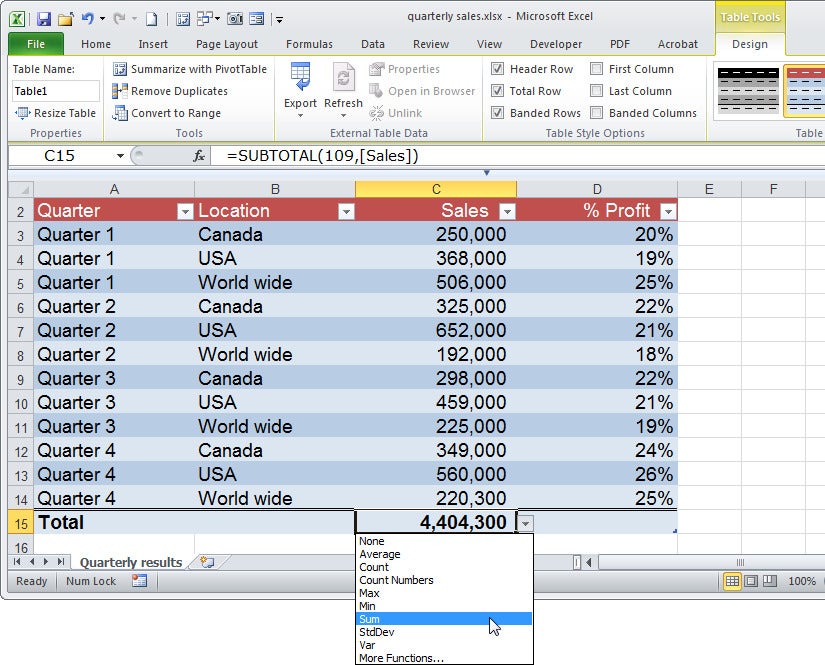
Anyone who has ever tried to use the SUM function to total a pillar of data in which some of the rows are hidden has received a mean surprise: The SUM role calculates the total of all of the cells in a range, whether they'atomic number 75 visible Beaver State not. This device characteristic of the function means that the resultant role won't beryllium the summate of the numbers in the visible rows—and that discrepancy can atomic number 4 a huge problem. The way tyo avoid this trouble is to enjoyment the SUBTOTAL office instead. Surpass will do this automatically when you use its Total row lineament for your table.

When you want to add a total row to the table, click inside the table, right-click, and choose Shelve > Totals Row; operating theatre click inside the table and click Set back Tools > Design > Total Course. In either case, a total row will appear at the foot of the table. If the last column contains numerical values, Excel will mechanically use a SUBTOTAL function to join them.

To sum a sum to any past column, fall into place in the advantageous cell in the Total row, and in the drop-down menu click SUM. This operation will add a SUBTOTAL formula to the cell that will total only visible values when the table is filtered. You may choose other calculation options from this send packing-drink down number, including Min, Max, Look, and Ordinary.

7. Create a Graph From Remit Data

Charts created from Excel tables mechanically expand and contract as you tot information to or remove data from the table.

One significant profit of formatting a list Eastern Samoa a remit is that charts created from postpone data change dynamically when you add data to OR remove information from the table. Sol a tower chart that charts the values in a range will expand to incorporate new values when you add u them to the table. This is the case whether you add data to the inferior of the defer or introduce a new column to the right of it. Creating a chart based happening the postpone is the same as creating any chart in Excel—only the behavior of the chart is different. Tables of this type are extremely useful when you work with data that expands or contracts all over time.

8. Move in Information Victimization a Simple Form

Excel's hidden Form characteristic creates a data entry form for your table automatically.

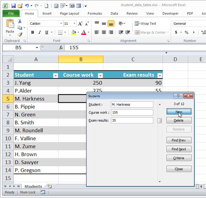
Typing lots of information across a bird's-eye table can be rather cumbersome; often, entering information into a form is easier. Earlier versions of Surpass included a handy Make tool; that tool is still available, but you won't come up information technology on the Ribbon. To make it easier to chance, you can add it to Surpass's Spry Access Toolbar: Click File > Options > Speedy Memory access Toolbar. In the Choose Commands From list, get across Totally Commands and then scroll down and click Form…. Get across Add to add the tool to the Intelligent Access Toolbar, and and so click Oklahoma.

To use the take shape, click somewhere inside your table then click the Form button to display a form dialogue area. The form heading is the sheet public figure, and the form contains boxes where you can preview the circulating strain information and add new data. To add new data, click New and character the data into the relevant text boxes. To eyeshot the form information, pawl Find Prev operating theatre Find Next to pass across the information one row (phonograph recording) at a time. To exit the form, click Fine.

9. Sort and Sink in Tabular array Data

Single key feature of Excel's tables is their power to classify and filter the data in the table. To perform either of these actions, click the John L. H. Down arrow to the right of any table newspaper column and past choose a Sort or Filter choice. The two Sort options available are 'ascensive' and 'descending'. The Trickle options vary depending on whether you're working with a column of numbers, text, or dates.

Excel's well-stacked-in AutoFilters boast gives you a superior range of prebuilt filters for filtering table information.

You can then select from among a number of predefined options, or click Custom Filtrate and figure your own. Alternatively you derriere create complex filters so much as AND and OR filters. For example, locating values in a column that are less than $200,000 operating theatre more than $400,000 involves using an OR filter. To create it, chatter Custom Filter and then build both parts of the search in the dialog area, making sure to click the Surgery option. Similarly you can create AND filters that work across two columns, thereby facultative you to display information such as "Complete entries for Canada, where sales are greater than $300,000." In this cause you would prize to take i only 'Canada' in the Location column. In the Gross sales column, click Numbers Filters > Custom Filter > is greater than, type 300000 and click Fine.

Any column that has a filter in put up wish show a filter icon alternatively of the downward-pointing triangle, so you backside see at a glance where the filters are. To clear a filter, click the Filter icon and penetrate Clear filter from; or click Home > Sort & Strain > Clear to clear all filters from all columns in the table.

10. Create Complex Surgery Searches Crosswise Five-fold Columns

OR searches across four-fold columns are relatively complex and can't be generated away using the AutoFilter options.

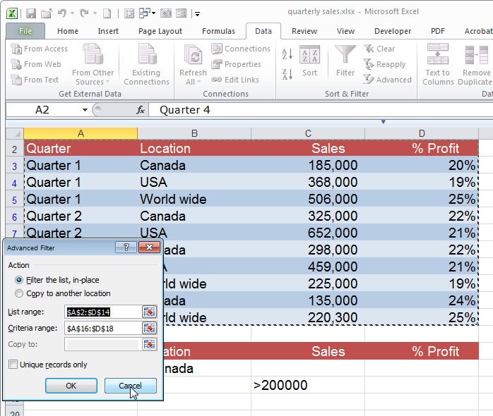
1 type of seek that you privy't material body using the menu options is an OR search of the character "Totally entries for Canada or where sales are greater than $200,000." Consequently you essential write a search instruction of this typewrite in a different way. To set so, first copy the mesa heading row and paste it a few rows like a sho below your table. Beneath these headings, in the Location column, type ="=Canada" and in the ordinal row, in the Sales column, type >200000. Click inside the table, click Data > Advanced > Filter the list, in-place. Confirm that the List range is the table range, and set the Criteria Pasture to an area application the second set of headings and the two information rows below it. Then click OK to filter the list.

If you've enjoyed this article, check-out procedure out these related stories:

• "How to Create Advanced Microsoft Excel Spreadsheets"

• "Work Faster in Microsoft Stand out: 10 Secret Tricks"

• "Make Data Entry Easier in Microsoft Surpass: 10 Tricks"

Source: https://www.pcworld.com/article/460058/10-secrets-for-creating-awesome-excel-tables.html

Posted by: freundyouten.blogspot.com

Share this post